In Finite Element Method, the discussion often begins with something called as statement of weighted residuals. So let us explore what it means to me.
Some background
Let us say we have a differential equation given by \eqref{eq:gde} with boundary condition as $y = 0$ at $x = 0$ and let us restrict ourselves to the domain $x \in [0, 1]$. \begin{equation} \dfrac{\mathrm{d}y}{\mathrm{d}x} = 3 x^{2} \label{eq:gde} \end{equation}
Solution of this differential equation can be obtained very easily by integrating both sides and then eliminating the constant term using boundary condition. The exact solution is given by \eqref{eq:gde-sol}. \begin{equation} y = x^{3} \label{eq:gde-sol} \end{equation} We will be using this differential equation and referring to the exact solution throughout this article.
Approximate solution and domain residual
Now lets just pretend that the differential equation given by \eqref{eq:gde} is either too complex to solve analytically or it has no exact solution. So the only option left to us is to solve it using some numerical technique which should give us an approximation to the actual solution i.e. \eqref{eq:gde-sol}.
Before we proceed with the numerical solution, lets see what information do we have about the approximate solution which we want to find out.
- The approximate solution should satisfy differential equation given by \eqref{eq:gde} at each point inside the domain i.e. $x \in (0, 1)$.
- The approximate solution should satisfy the condition $y = 0$ at $x = 0$, i.e. at the boundary of the domain.
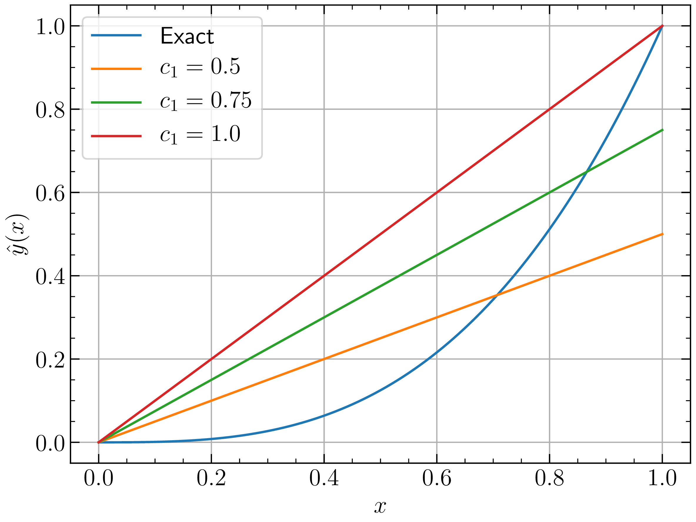
For the sake of brevity, lets say the approximate solution is $\hat{y}(x)$ which is an approximation to $y(x)$. Of the two conditions above, second one seems easy to satisfy. Can we come up with some function $\hat{y} (x)$ which has property $\hat{y} = 0$ at $x = 0$? How about $\hat{y} (x) = c_1 x$, where $c_{1}$ is an arbitrary constant? Does this function satisfy the first condition given above? Definitely not. But I still want to use the same function as an approximation to the exact solution given by \eqref{eq:gde-sol}. There is an issue though, I do not have any idea about what should be the arbitrary constant $c_{1}$. With change in $c_{1}$, the function $\hat{y} (x)$ also changes. So lets plot $\hat{y} (x)$ for different values of $c_{1}$ and on the same plot we will also show the analytical solution just for the sake of comparison.

From above figure, it is clear that none of the $c_{1}$ values are giving us an approximation which satisfies condition 1. I can say this only because I have the exact solution with me. In reality, you will never have the exact solution to compare with. In fact, if you already have the exact solution, seeking an approximate solution is stupid. So lets continue with our stupidity.
As I dont know the exact solution I want to use $c_{1} x$ as our approximate solution. But what value of $c_{1}$ should I choose which will keep $\hat{y} (x)$ as close to actual solution as possible? How to decide which curve is better than all the other infinite choices? This is where we are going to use our first condition which states that the actual solution satisfies \eqref{eq:gde} at each point on the domain. However, we have an approximation $\hat{y} (x)$ which does not satisfy the differential equation at every point in the domain. If we substitute $\hat{y} (x)$ into the differential equation, what we get is error $R_{\Omega}$. The error $R_{\Omega}$ is often referred to as domain residual as this gives us the residual (i.e. error) at any point in the domain. \begin{eqnarray} \label{eq:residual} \dfrac{\mathrm{d} \hat{y} (x)}{\mathrm{d} x} - 3 x^2 & = & R_{\Omega} \nonumber \end{eqnarray}
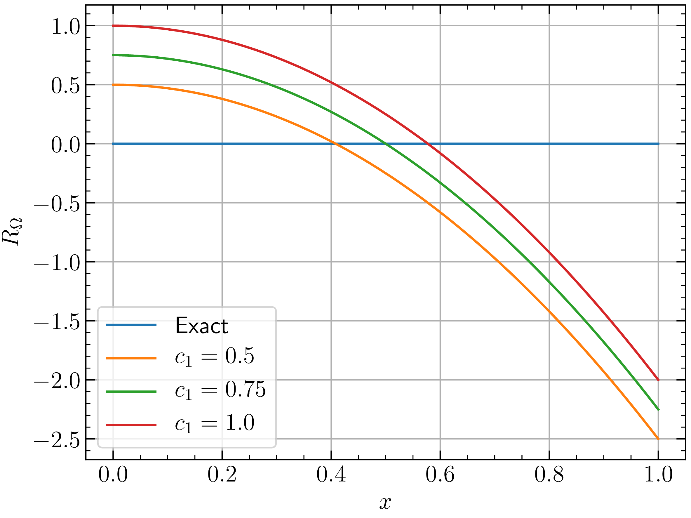
If we substitute \(x\) coordinate of any point in the domain, we will get error at that point due to approximation function \(\hat{y} (x) = c_1 x\). For ex: @ \(x = 0\), the domain residual is \(c_1\) and @ \(x = 1\) the domain residual is \(c_1 - 3\). One can also note that @ \(x = \sqrt{\dfrac{c_1}{3}}\), the domain residual vanishes.
Minimize residual
We have seen that the approximation function introduces domain residual at each point on the domain. Also the domain residual varies from point to point and at some point it can also be zero. Ideally we want the domain residual to be zero at all points. But as that is not possible, let's do whatever best we can. Let's just have one more plot for varying value of \(c_1\). But this time instead of plotting the approximation function, lets plot the domain residual. We know \(R_{\Omega}\) is given by \begin{equation} R_{\Omega} = c_1 - 3 x^2 \nonumber \end{equation}

One of the easiest ways to minimize this error is using method of least squares. This time even though we do not have exact solution, we do have domain residual which is equivalent to error. However, we will not discuss that here. We want to see method of weighted residuals in action to minimize this residual. But before minimizing it, lets try to visualize it in a graphical way.
Graphical representation of domain residual ($R_{\Omega}$)
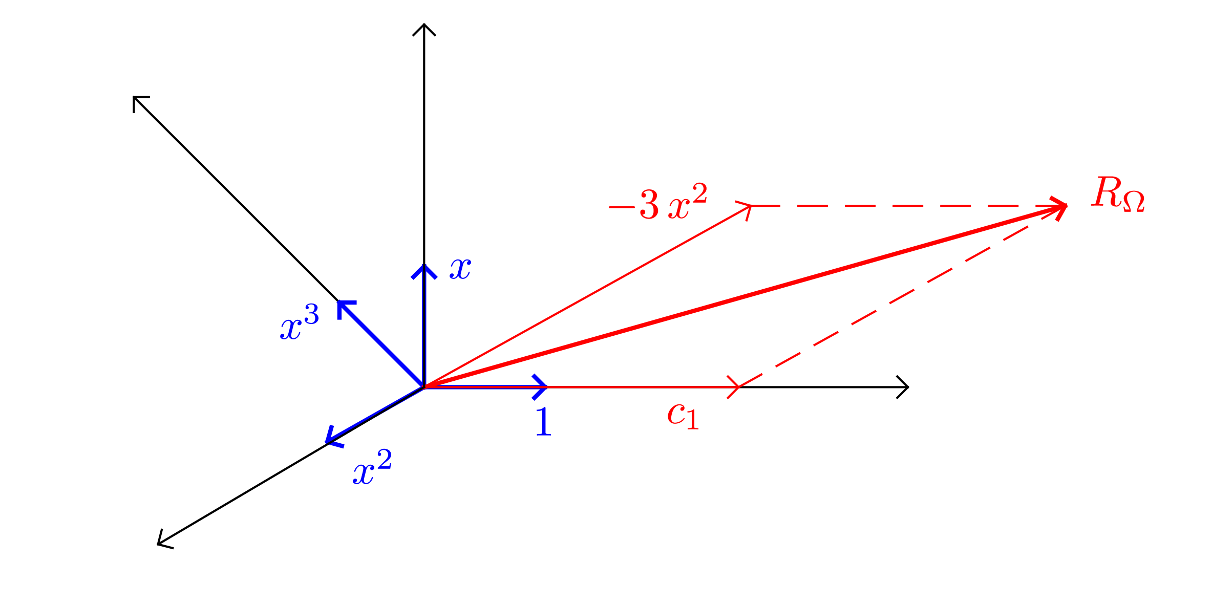
We know that the exact solution is \(y (x) = x^3\). I can write the same expression as \begin{equation} y (x) = a_0 + a_1 x + a_2 x^2 + a_3 x^3 \nonumber \end{equation} Where \(a_0 = a_1 = a_2 = 0\) and \(a_3 = 1\). We will look at this expression just like we look at vectors. Lets say the function \(y (x)\) is composed of four basis functions, \(1, x, x^2 \text{ and } x^3\) weighted by \(a_0, a_1, a_2 \text{ and } a_3\) respectively. Note that the basis functions need not be orthogonal to each other. So lets just draw this (conceptually only). Let me emphasize that the below drawing is only for understanding. It is based on concepts of vector spaces which are applicable in function spaces as well. However we cannot draw function spaces like this (or at least that's what I think).

Above figure shows a conceptual visualization of domain residual. The function space contains four basis vectors \(1, x, x^2 \text{ and } x^3\). Each point in this function space represents a polynomial of degree \(3\). So in the same function space we can draw our exact solution \(y (x) = x^3\) and the domain residual \(R_{\Omega} = c_1 - 3 x^2\). We can take inner product of \(R_{\Omega}\) with each of the basis function to get its projection on that basis function. As we want \(R_{\Omega}\) to vanish, we will enforce each inner product to vanish. The inner product of two functions \(u (x) \text{ and } v (x)\) is given as
\begin{align} \langle u, v \rangle = \underset{\Omega}{\int} u (x) v (x) \mathrm{d} x \nonumber \end{align}
So the inner product of \(R_{\Omega}\) with four basis functions is given as
\begin{align} \langle 1, R_{\Omega} \rangle &= \underset{0}{\overset{1}{\int}} R_{\Omega} \mathrm{d} x \label{eq:wr1}\\ \langle x, R_{\Omega} \rangle &= \underset{0}{\overset{1}{\int}} xR_{\Omega} \mathrm{d} x \label{eq:wr2}\\ \langle x^2, R_{\Omega} \rangle &= \underset{0}{\overset{1}{\int}} x^2 R_{\Omega} \mathrm{d} x \label{eq:wr3}\\ \langle x^3, R_{\Omega} \rangle &= \underset{0}{\overset{1}{\int}} x^3 R_{\Omega} \mathrm{d} x \label{eq:wr4} \end{align} Each inner product is set to 0, which gives us four conditions. In this particular problem, our chosen approximation is linear and hence it has only one constant \(c_1\). Hence we do not need all the four conditions. Here we only need one condition. So we can pick any of the four conditions. I am goint to take two conditions and find out approximate solution in each case.
Method of weighted residuals
Finally we are here! Have a look at \eqref{eq:wr1}-\eqref{eq:wr4}. What is happening there? We have a domain residual term \(R_{\Omega}\). And instead of integrating that term over the domain, we are first weighting that term by one of our basis functions and then integrating over the domain. The final part is to set this integral to zero. This itself is nothing but weighted residuals. And obtaining the approximation using this is nothing but Method of Weighted Residuals;. So lets just proceed with finding out a better approximation.
Weighting function = 1
The weighted residual becomes \begin{eqnarray} \langle 1, R_{\Omega} \rangle & = & \underset{0}{\overset{1}{\int}} R_{\Omega} \mathrm{d} x \nonumber \\ & = & \underset{0}{\overset{1}{\int}} (c_1 - 3 x^2) \mathrm{d} x \nonumber \end{eqnarray}
Set the residual to zero.
\begin{eqnarray} 0 & = & \underset{0}{\overset{1}{\int}} (c_1 - 3 x^2) \mathrm{d} x \nonumber \\ & = & [c_1 x - x^3]_0^1 \nonumber \\ & = & c_1 - 1 \nonumber \\ \operatorname{Hence} \quad c_1 & = & 1 \nonumber \end{eqnarray} So the approximation function is $\hat{y} (x) = x$.
Weighting function = $x$
The weighted residual statement is
\begin{eqnarray} \langle x, R_{\Omega} \rangle & = & \underset{0}{\overset{1}{\int}} xR_{\Omega} \mathrm{d} x \nonumber \\ 0 & = & \underset{0}{\overset{1}{\int}} x (c_1 - 3 x^2) \mathrm{d} x \nonumber \\ & = & \left[ \dfrac{c_1 x^2}{2} - \dfrac{3 x^4}{4} \right]_0^1 \nonumber \\ & = & \dfrac{c_1}{2} - \dfrac{3}{4} \nonumber \\ \operatorname{Hence} \quad c_1 & = & 1.5 \nonumber \end{eqnarray}
This time the approximation is $\hat{y} (x) = 1.5 x$
So what is the approximation function \(\hat{y} (x)\), if remaining two basis functions are used for weighting? I keep it as an exercise for you.
This conceptually completes our problem. However, lets just have a look at our approximation and exact solution. We can definitely say that the approximations are not appropriate. Why? Because our initially assumed \(\hat{y} (x) = c_1 x\) is a poor choice. The differential equation contains first order derivative and it equates with a quadratic term in \(x\). This itself tells us that the solution has to be cubic. So what happens if we choose a cubic polynomial as an approximation? Lets find out quickly.
Generic approximation function
let \(\hat{y} (x) = c_0 + c_1 x + c_2 x^2 + c_3 x^3\). We need to find out the values of constants \(c_{i = 0, \ldots, 3}\). Based on boundary condition \(y (0) = 0\), we can eliminate \(c_0\) as it has to be zero. So \begin{eqnarray} \hat{y} (x) & = & c_1 x + c_2 x^2 + c_3 x^3 \nonumber \\ \dfrac{\mathrm{d} \hat{y}}{\mathrm{d} x} & = & c_1 + 2 c_2 x + 3 c_3 x^2 \nonumber \end{eqnarray}
Substituting in \eqref{eq:gde} \begin{eqnarray} c_1 + 2 c_2 x + 3 c_3 x^2 & = & 3 x^2 \nonumber \\ \operatorname{Hence} \quad R_{\Omega} & = & c_1 + 2 c_2 x + 3 c_3 x^2 - 3 x^2 \nonumber \end{eqnarray} Just by looking at above equation we can say that \(c_1 = c_2 = 0\) and \(c_3 = 1\). But lets just follow our procedure to see what values we come up with.
Our approximation function \(\hat{y} (x)\) contains three arbitrary constants. Hence we need three conditions i.e. three basis functions as weighting functions. So as per the method of weighted residuals, lets choose \(x, x^2 \text{ and } x^3\) as the weighting functions.
\begin{align} \langle x, R_{\Omega} \rangle &= \underset{0}{\overset{1}{\int}} x (c_1 + 2 c_2 x + 3 c_3 x^2 - 3 x^2) \mathrm{d} x \nonumber \\ 0 &= \left[ \dfrac{c_1 x^2}{2} + \dfrac{2 c_2 x^3}{3} + \dfrac{3 c_3 x^4}{4} - \dfrac{3 x^4}{4} \right]^1_0 \nonumber \\ &= \dfrac{c_1}{2} + \dfrac{2 c_2}{3} + \dfrac{3 c_3}{4} - \dfrac{3}{4} \label{eq:simEq1}\\ \langle x^2, R_{\Omega} \rangle &= \underset{0}{\overset{1}{\int}} x^2 (c_1 + 2 c_2 x + 3 c_3 x^2 - 3 x^2) \mathrm{d} x \nonumber\\ 0 &= \left[ \dfrac{c_1 x^3}{3} + \dfrac{2 c_2 x^4}{4} + \dfrac{3 c_3 x^5}{5} - \dfrac{3 x^5}{5} \right]^1_0 \nonumber\\ &= \dfrac{c_1}{3} + \dfrac{c_2}{2} + \dfrac{3 c_3}{5} - \dfrac{3}{5} \label{eq:simEq2}\\ \langle x^3, R_{\Omega} \rangle &= \underset{0}{\overset{1}{\int}} x^3 (c_1 + 2 c_2 x + 3 c_3 x^2 - 3 x^2) \mathrm{d} x \nonumber\\ 0 &= \left[ \dfrac{c_1 x^4}{4} + \dfrac{2 c_2 x^5}{5} + \dfrac{3 c_3 x^6}{6} - \dfrac{3 x^6}{6} \right]^1_0 \nonumber\\ &= \dfrac{c_1}{4} + \dfrac{2 c_2}{5} + \dfrac{c_3}{2} - \dfrac{1}{2}\label{eq:simEq3} \end{align}
solving eqs. \eqref{eq:simEq1}, \eqref{eq:simEq2} and \eqref{eq:simEq3} simultaneously, we get \begin{eqnarray} c_1 & = & 0 \nonumber \\ c_2 & = & 0 \nonumber \\ c_3 & = & 1 \nonumber \end{eqnarray}
So the approximation is
\begin{eqnarray} \hat{y} (x) & = & x^3 \nonumber \end{eqnarray}
We were very fortunate to have our approximation turn out to be the exact solution. This seldom happens in reality and hence we should always treat the solution obtained as an approximate one for further processing.
Points to ponder
In the discussion above, we have set the inner product of some function $\phi(x)$ with domain residual $R_\Omega$ to zero, where, $\phi(x)$ is an arbitrarily chosen basis function. So, essentially we are completely eliminating the domain residual along all the chosen basis functions. Yet, we call this minimization and not elimination of $R_\Omega$. Can you see why? Do let me know in the comments.
Summary
In this article we learned
- What is domain residual?
- Conceptual representation of the weighted residual
- Obtaining approximation using weighted residuals
